Data Collection
Classroom experiments can not only be a fun way for children to learn about the world around them, but also a great opportunity to develop data collection techniques. There are two main types of data: quantitative and qualitative. To learn more about these types of data, see our article on different types of data or click on the section below for a summary.
Click here to learn about the different types of data
Quantitative data can be recorded using a number. This data could be discrete, taking only specific values from the real numbers, such as whole numbers. Some quantitative data can be continuous, taking any value from the real numbers.
The other type of data we can collect is qualitative data. This is non-numerical data, such as a person’s favourite animal or the colour of a car.
Different types of data can be collected and recorded in different ways.
To showcase the different types of graphs, we will use the pretend data, which you can see below. This includes some children’s height, shoe size and favourite animal.
Click here to see the data
Data of a pretend sample of students:
| Height (cm) | Shoe Size | Favorite Animal |
|---|---|---|
| 106.3 | 8.5 | dog |
| 99.1 | 7.5 | cat |
| 106.7 | 9 | hamster |
| 109.5 | 11 | dog |
| 95.8 | 7 | cat |
| 104.4 | 8 | dog |
| 108.9 | 10 | dog |
| 109.3 | 10.5 | cat |
| 99.4 | 7 | hamster |
| 102.2 | 9 | dog |
| 105.5 | 8.5 | cat |
| 106.9 | 10 | dog |
| 109.5 | 10 | hamster |
| 100.7 | 9 | cat |
| 95.1 | 7.5 | dog |
| 104.4 | 9.5 | hamster |
| 105.3 | 9.5 | dog |
| 95.9 | 7 | cat |
| 109.9 | 10.5 | dog |
| 94.2 | 7 | dog |
Tallies
Qualitative (not a number) data is often recorded using tallies or tables. A tally is shown below. Here we add a mark in the correct row for each person’s favourite animal. When we reach \(5\) marks, we strike through the first \(4\) and then repeat this process so the tallies are grouped in multiples of five. Grouping the tallies in this way makes them easier to compare and count quickly.
| Favorite Animal | Tally | Frequency |
|---|---|---|
| Dog | \(\cancel{////}\cancel{////}\) | 10 |
| Cat | \(\cancel{////}/\) | 6 |
| Hamster | \(////\) | 4 |
We have added an extra column to record the frequency, which is the sum of the tallies and can be filled in once we have finished collecting the data. A table with just the frequency column is called a frequency chart.
Quantitative data can be recorded in this way, too, if it is grouped into bins. Below is an example of this where the heights of the children in the data have been grouped into categories \(2\)cm wide.
| Height (cm) | Tally | Frequency |
|---|---|---|
| 93 - 95 | \(/\) | 1 |
| 95 - 97 | \(///\) | 3 |
| 97 - 99 | 0 | |
| 99 - 101 | \(//\) | 3 |
| 101 - 103 | \(/\) | 1 |
| 103 - 105 | \(//\) | 2 |
| 105 - 107 | \(\cancel{////}\) | 5 |
| 107 - 109 | \(/\) | 1 |
| 109 - 111 | \(///\) | 4 |
Here, a value of \(99\) would have to be treated carefully as it is on the boundary of two categories. Normally, we round up and would include this in the category \(99-101\).
In the image below a child has made their own tally marks.

Tables
If we have more than one category we want to count, we can do so with a table. In the table below, we record both the shoe sizes of the children and their favourite animal. This is called a two-way table. Often, including row and column totals can help check that all the data has been included correctly; the sum of the rows should equal the sum of the columns.
| Favorite Animal/Shoe Size | 7 - 9 | 9 - 11 | Total |
|---|---|---|---|
| Dog | 4 | 6 | 10 |
| Cat | 4 | 2 | 6 |
| Hamster | 1 | 3 | 4 |
| Total | 9 | 11 | 20 |
Stem and Leaf Plots
A more complex method for recording quantitative data is stem and leaf plots. In the stem and leaf plot below, we record the heights of the children in our data. Here \(109|3\) means \(109.3\).

Once collected, data can then be displayed in different ways. To see some of these ways, see our article on different types of graphs.